Quantum Kolmogorov-Arnold Networks for top quark jet tagging

A technical summary of the QKAN project, Google Summer of Code 2026 at ML4SCI

This project was developed by Jorge Toral and can be found in this GitHub repository.

---

1. The problem and the core idea

At the Large Hadron Collider, a top quark decays almost instantaneously and produces a jet (a collimated spray of particles) with a characteristic internal substructure, distinct from that of an ordinary jet originating from a light quark or a gluon (QCD). Distinguishing these two types of jet, a task known as top tagging, is a well-studied binary classification problem, with classical reference architectures reaching AUCs above 0.96-0.98 on the public dataset used in this project (Kasieczka et al., 2019): jets simulated at 14 TeV with Pythia8 and an ATLAS-like Delphes detector card, reconstructed with anti-$k_T$ and $R=0.8$ in the range $p_T \in [550, 650]$ GeV.

The goal of the project is to answer a question other than outperforming those architectures: can a variational quantum neural network (VQC) perform this task, and what role can a classical network play in making it feasible?

The underlying limitation is the cost of simulating a quantum circuit, which grows as $O(2^Q)$ with the number of qubits $Q$. Feeding a jet with dozens of variables directly into a VQC is impractical. The solution explored here uses a classical Kolmogorov-Arnold Network (KAN) as a preprocessor and qubit filter: it is trained, pruned down to a small, interpretable topology, and that pruned topology determines how many qubits the quantum circuit needs and how they are connected. In this way, the classical model sets the quantum resource systematically, without resorting to trial and error.

The full pipeline, documented across three notebooks (EDA_top.ipynb, Training_process.ipynb, Analysis_of_results.ipynb), preprocesses the jets into balanced replicas, trains and prunes the KAN, extracts each surviving edge into a compact basis (Chebyshev or sine) as a warm start, fine-tunes the QKAN on an ideal simulator, on one with finite-shot noise, and on one with hardware noise, and compares everything against a classical Random Forest.

2. Motivation for the KAN architecture

Kolmogorov-Arnold Networks, proposed by Liu et al. (2024) building on the Kolmogorov-Arnold representation theorem (KAT), invert the design of a traditional multilayer perceptron (MLP). In an MLP, the activation functions are fixed (ReLU, tanh, …) and live on the nodes; the learnable weights are scalars on the edges. In a KAN the relationship is inverted: each edge carries its own learnable univariate function, parameterized as a spline, and the nodes only sum. The KAT theorem guarantees that any continuous multivariate function can be written as

\[f(x_1, \dots, x_n) = \sum_{q=1}^{2n+1} \Phi_q\left(\sum_{p=1}^{n} \phi_{q,p}(x_p)\right)\]

that is, as a composition of univariate functions and sums. Two properties follow that this project exploits directly. The first is interpretability: once training is finished, each edge can be fit symbolically against a library of candidate functions, giving a closed-form expression for the transformation it performs. The second, crucial for this project, is structured prunability: since each edge is an independent functional unit, an attribution (how much it contributes to the output) can be measured and the edge removed if negligible, without breaking the interpretation of the rest of the network.

A follow-up work by the same authors, KAN 2.0 (Liu et al., 2024), also introduces multiplication nodes. The KAT theorem in its classical form only guarantees composition through sums; allowing some hidden nodes to multiply their inputs expresses variable interactions directly. This project’s classical architecture (HEPKAN, a subclass of pykan) adopts this idea and uses a hidden layer with sum and multiplication nodes in parallel.

3. Data exploration: what distinguishes a top jet

Before training, the EDA notebook characterizes the dataset. The HDF5 file does not document the order of its columns, so it was inferred from the data: each block of four columns corresponds to one constituent particle of the jet, with energy in the first position and the three momentum components afterward. The pattern is recognizable in the column means, which are much larger in the first column of each block of four.

Four observations emerged from the histograms and radial profiles and guided the subsequent design:

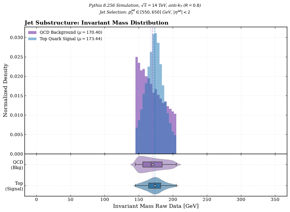
• Invariant mass discriminates, but isn’t enough. $m_{jet} = \sqrt{E^2 - p_x^2 - p_y^2 - p_z^2}$ has a clear peak in the signal around the top quark mass (~173 GeV), while the background is wider. The two distributions overlap by sections, so the 145-205 GeV window was selected for all experiments: within it, the trivial mass cue is largely removed and classifiers must rely on subtler information.
• Top jets are more populated: multiplicity (number of constituents) is systematically higher and more spread out than in QCD, consistent with a three-body decay, for this selected mass window.
• Top jets are more diffuse: the radial energy profile and the cumulative $p_T$ fraction grow more gradually in tops than in QCD, where energy is more concentrated near the jet axis.
• $\eta$-$\phi$ scatter plots were inconclusive due to noise and scale.

An artifact was also detected: the $\Delta R$ distribution does not show the expected sharp cutoff at 0.8, due to a small constant added to avoid division by zero. Constituents outside the jet radius were filtered out to correct it.

From this the input representation was built, combining global variables (jet mass and multiplicity, counting only constituents with energy above $10^{-8}$) with local variables for each retained constituent ($\Delta R$ to the jet axis and $p_{T,\text{rel}}$). Using the 80% cumulative $p_T$ criterion, around 15 constituents were estimated to suffice to capture most of the energy. The final pipeline uses only the 10 most energetic constituents per jet, for a total of 22 inputs (2 global + 10 pairs of local variables). Each original jet carries up to 200 stored constituents; the cut to 10 is a deliberate compression decision revisited in the results and conclusions, since the model never sees 95% of the particles recorded by the detector.

The local variables already live in $(0,1)$. The global ones undergo a logarithmic transform followed by tanh normalization, deliberately keeping the outliers: the centers of the two class distributions are similar and the discriminative information lies in the tails.

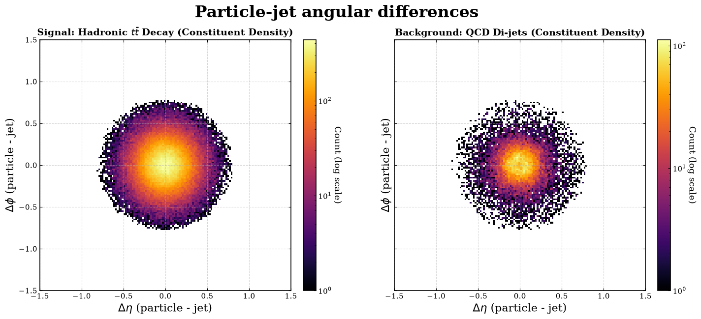
Finally, since the number of events in the mass window differs between classes (there are more tops), the majority class is subsampled to balance it, and the result is split into 5 disjoint, class-balanced subsets. Each seed selects one (seed % 5), so several seeds produce independent end-to-end replicas rather than a single point estimate.

4. The classical architecture and its pruning

The classical model has architecture [22, [9, 9], 1]: 22 inputs, one hidden layer with up to 9 sum nodes and 9 multiplication nodes in parallel, and a scalar output. The B-splines use degree $k=3$ and grid size 5, for a total of 8,568 parameters. In the reference run (seed 10), the base model reached a test AUC of 0.792 in the point evaluation reported in the notebook, consistent with the mean of 0.789 ± 0.002 obtained by aggregating the five replicas (section 8). Training stopped early, around epoch 20 of the planned 60.

HEPKAN introduces three practical modifications over pykan, motivated by the project’s limited computational resources: a fix for a bug in prune_input (it passed a module instead of a string name when rebuilding the pruned model, which broke checkpoint serialization), a plotting routine that reuses a single Matplotlib figure for all edges and skips already-pruned ones, and a no-op history logger that avoids writing a checkpoint on every model mutation during pruning and symbolic search.

Pruning combines an input threshold of 0.01 with attribution thresholds of 0.04 (nodes) and 0.06 (edges), and adds a hard constraint aimed at the quantum limit: a fan-in cap of two, which keeps only the two strongest input edges per hidden neuron. After pruning, the structure is retrained for 20 epochs; in the reference run (seed 10), validation AUC rises from 0.714 to ~0.755.

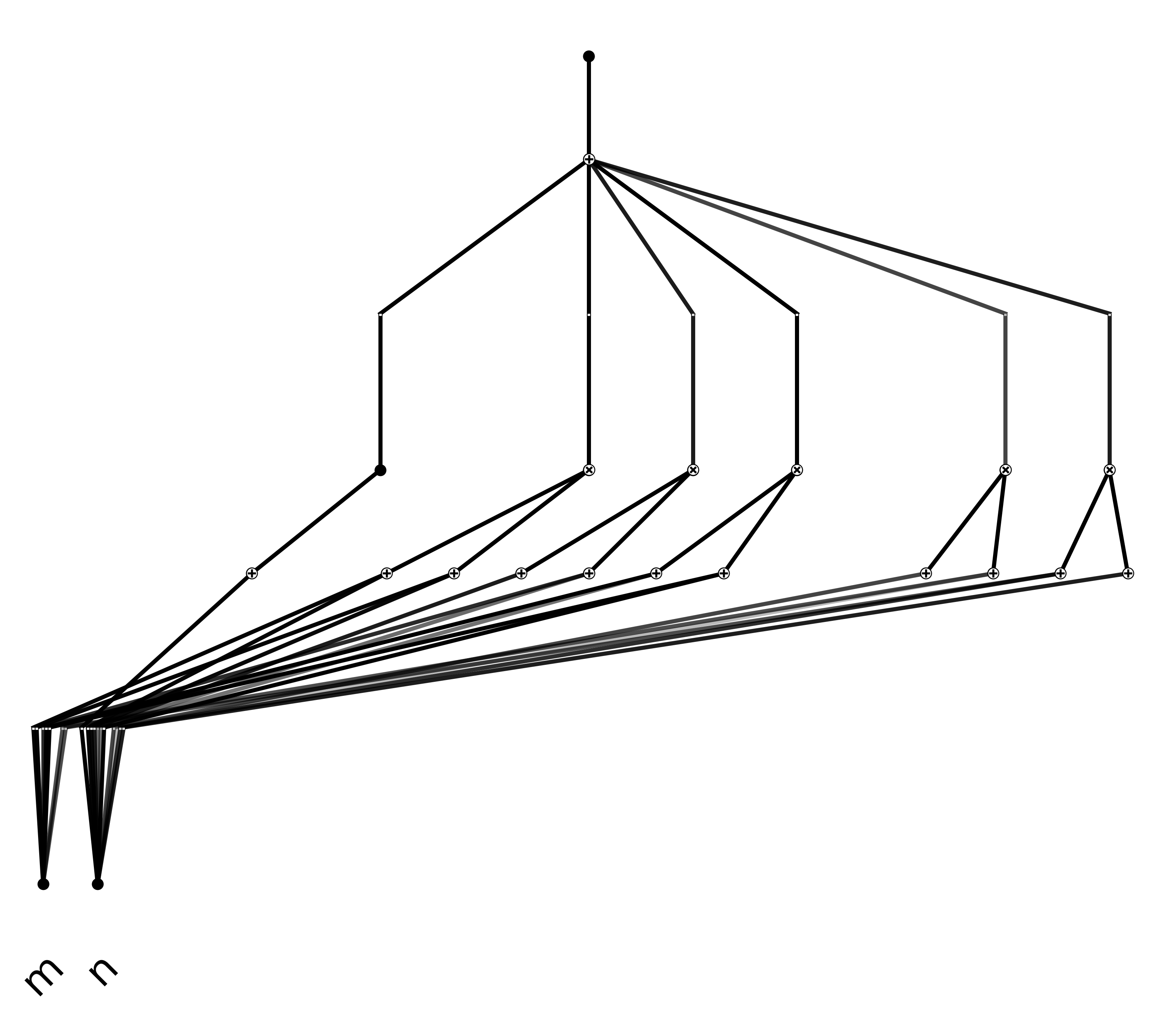
The result for the reference run is very compact: of 22 input variables, only 2 survive (jet mass and multiplicity), organized into 1 sum node and 5 multiplication nodes. This finding agrees with the feature importance (MDI/Gini) of the reference Random Forest (section 7), which independently also points to mass and multiplicity as the most predictive variables among the 22 available. This cross-check indicates that aggressive pruning preserves the relevant signal. The pattern repeats across all five seeds: mass and multiplicity always survive, with 10 or 11 qubits depending on the seed (in seeds 11 and 12 no sum node survives).

The notebook also runs a symbolic fit on each surviving edge, matching it against a library of candidate functions to obtain a formula-based interpretation. This is the main interpretability advantage of KANs and belongs to the project’s purely classical branch. The quantum branch uses the numerical response of each edge instead of the symbolic formula.

5. From the classical graph to the quantum circuit

An extractor isolates the response of each active edge by disconnecting the other inputs to its destination node, and exports a serialized graph of sum and multiplication nodes. For the reference run, that graph has 11 qubits, 18 input edges, 5 IsingZZ transfers, and 6 output edges, a direct result of compressing 22 variables into 2 surviving inputs distributed across 1 sum node and 5 multiplication nodes. Qubits are counted per surviving accumulator node: the same input variable can be re-uploaded onto several wires if it feeds several different hidden nodes. This is why 2 variables occupy 11 qubits.

The circuit follows five design principles:

1. Data re-uploading: each edge’s univariate function is modeled through repeated $R_y$/$R_z$ rotations of the input data, parameterized by the coefficients fitted in the warm start, rather than encoding the data once.
2. Inherited topology: the classical hidden layer decides which variables matter and how many qubits are used; the circuit reproduces the topology of the pruned graph.
3. Summation: each edge feeding a sum node chains consecutive $R_Y$ and $R_Z$ rotation gates on the same wire, so sum nodes require no two-qubit gate at all. The number of re-uploads depends on the degree of the polynomial fitted on the edge. For this work, a fixed degree of 4 was used.
4. Multiplication: implemented with an IsingZZ gate combined with a CNOT, the only point in the circuit that introduces entanglement between wires.
5. Single-qubit readout: all information collapses onto one output wire, and the prediction is the Pauli-Z expectation value of that qubit, passed through a sigmoid to obtain a class probability.

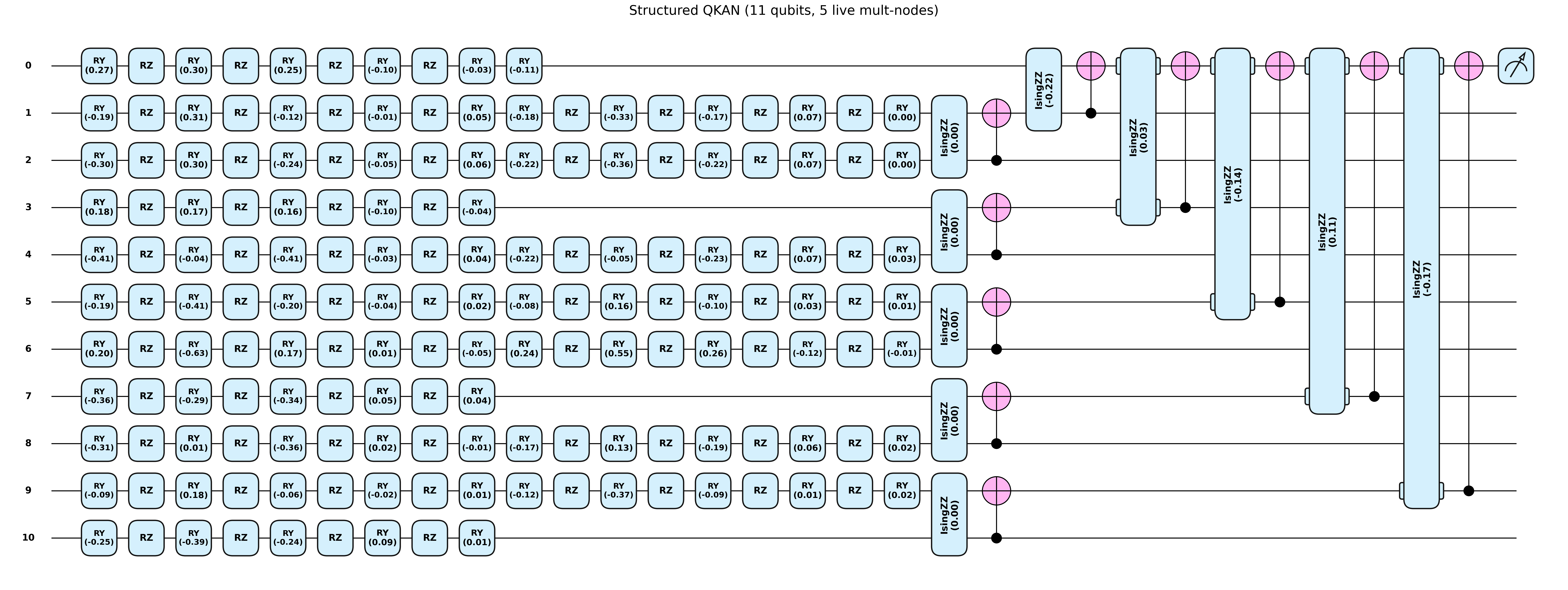
The hidden-to-output stage is a variational readout and does not literally reproduce a second KAN layer, because a hidden node’s value lives in a qubit’s phase and cannot be re-uploaded without an intermediate measurement. For this reason only depth-2 networks are supported. This is an explicit design limitation, also motivated by the barren plateau risk of stacking re-uploading layers (Arias Alamo et al., 2025), and it remains as future work.

The model can run on three simulators, representing successively more realistic versions of the same circuit: ideal (lightning.qubit, with no noise or finite sampling), shots (default.qubit with a finite number of shots, which introduces the statistical noise of a real measurement), and noisy (Qiskit Aer with a noise model derived from FakeManilaV2, which additionally simulates the decoherence and gate error of a specific IBM device). FakeManilaV2 models ibmq_manila, a real 5-qubit device, while the reference circuit uses 11: the first 5 are modeled with the FakeManilaV2 noise and the rest are modeled as ideal.

Training uses binary cross-entropy with logits, the Adam optimizer, and a ReduceLROnPlateau scheduler that halves the learning rate when validation stalls. Simulation is expensive: averaged over the five seeds, the noisy backend takes about 2,460 s per full evaluation, versus ~135 s on ideal, a difference of about 18 times. Each epoch therefore trains on a fresh random subset (~1,000 samples) and validates on a fixed subset.

6. Circuit initialization: the warm start

Before fine-tuning the circuit with gradient descent, the initial angles must be set. Three strategies were compared.

Chebyshev. Each isolated edge response is fit as $y \approx \sum_{i=0}^{N} c_i T_i(x)$ over $[-1,1]$, following the design of Chebyshev-KAN (Sidharth et al., 2024), and the resulting coefficients are converted into the initial rotation angles. The degree is fixed at $N=4$ for all edges. The choice of a fixed degree instead of an adaptive one comes from a bug diagnosed during the project. The original approach searched for the smallest degree that exceeded an $R^2$ threshold, but that criterion almost always chose low degrees and produced inconsistent metrics, because the circuit lost the classical structure’s information. The symptom was an abrupt drop in reference AUC (from ~0.80 to 0.26-0.36) as the training set got smaller. The fit is not nested by degree: lowering the degree removes the high-order coefficients and also perturbs the low-order ones that remain. Reverting to a fixed degree restored the expected behavior, and the case is documented as one of the project’s findings.

Sine basis. As an alternative, a fixed-frequency sinusoidal basis was implemented, following the design of SineKAN (Reinhardt et al., 2025): $y \approx \sum_k A_k \sin(\text{freq}_k \, x + \text{phase}_k)$, with the amplitudes $A_k$ obtained via least squares over a fixed grid of frequencies and phases. In SineKAN, the notion of an edge’s “degree” corresponds exactly to the number of sine terms summed in that grid, that is, the number of accumulated sinusoidal harmonics, in contrast with the growing-degree polynomial of Chebyshev. This basis is also the one used by Ria Khatoniar in the classical-readout branch of her GSoC 2025 project (Khatoniar, 2025a, section 10), and the reference script used to faithfully port the frequency-and-phase grid construction (constants $A=0.9724$, $K=0.9884$, $C=0.9994$ from the original SineKANLayer) comes directly from her code.

With this fixed basis, the Chebyshev experiment was replicated at small scale, fitting real edges extracted from the pipeline with both bases and comparing their $R^2$. The result quantitatively confirms what theory suggests: over the 110 edges extracted across the five seeds, the sine basis fit is moderate, with a mean $R^2$ of approximately 0.56 (median 0.84), well below Chebyshev’s near-perfect fit (mean $R^2$ of 0.998). Without a constant term, the sine basis cannot represent static offsets and produces negative $R^2$ on some edges.

To further verify this hypothesis, we repeated only the least-squares fit (without the full circuit training pipeline), adding a constant term to the sine basis. The result confirms the cause: the fit’s $R^2$ improves, surpassing even that of the Chebyshev basis. This rules out other issues with the least-squares procedure, such as ill-conditioning of the fixed frequency grid, and attributes the original sine basis’s poor fit to the missing constant term. That said, this verification was limited to the edge-level fit; we did not re-run the full circuit with this extended basis, so we do not know whether the improved $R^2$ translates into a better initial AUC for the warm start. A more accurate fit for each edge does not automatically guarantee better classification downstream in the circuit, so this remains an open question.

This finding is consistent with a recent theoretical paper on the same basis: the “Sinusoidal Approximation Theorem for KANs” (Gleyzer et al., 2025) gives a constructive universal-approximation proof for sine-basis KANs, in the spirit of the original KAT. The theorem guarantees that, with enough terms and freedom to fit frequency and phase, a sine basis can approximate any continuous function. The result of this project shows that a fixed grid, without a constant term and with only $N=4$ harmonics, does not yet exploit that capacity.

Random initialization. As a control, the pruned topology is kept exactly (same qubits and connections) and each angle is sampled from $\mathcal{N}(0,1)$. This separates the value of the transferred classical knowledge from the value of the topology alone.

Clamp in cosine. Both the Chebyshev coefficients and the randomly initialized angles are converted into the corresponding $R_Z$ gate rotation angle by passing through an arccosine, i.e., $\theta = \arccos(\text{value})$, ensuring that the angles remain within the valid rotation range. Since arccosine is defined over $[-1,1]$, any value outside this range is clamped to the limits between [-0.9999, 0.9999]. The sine basis has its values within [-1,1], so the clamp is not applied.

7. Classical baseline: Random Forest

To calibrate the distance between the quantum approach and what is classically achievable, a Random Forest with 300 trees (maximum depth 35) and balanced class weights was added. Unlike the KAN pipeline, it receives the full 22 variables, unpruned. It uses the same metric keys as the KAN trainers, so all models are aggregated into a single results table.

8. Results

All per-run metrics are collected into a single Parquet table (65 rows across 5 seeds). All experiments use the mass cut and the five disjoint subsets: each seed (10-14) trains and evaluates every model on its own subset, so the five seeds act as replicas.

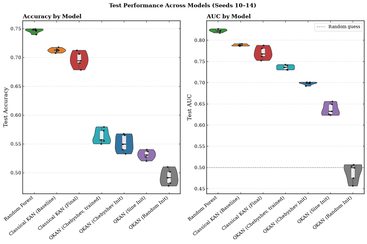
The following figure shows the per-seed distribution of test accuracy and AUC for seven representative models in the chain, from the Random Forest to the untrained, randomly initialized QKAN. The table summarizes the mean ($\pm$ standard deviation over 5 seeds) for all models.

Model	AUC (mean $\pm$ σ)	Accuracy (mean $\pm$ σ)	Background rejection at $\varepsilon_S=0.5$
Random Forest (22 features)	0.823 $\pm$ 0.004	0.746 $\pm$ 0.004	10.04 $\pm$ 0.57
Classical KAN, base	0.789 $\pm$ 0.002	0.712 $\pm$ 0.004	7.20 $\pm$ 0.37
KAN, retrained after pruning	0.756 $\pm$ 0.004	0.687 $\pm$ 0.005	5.81 $\pm$ 0.29
KAN, symbolic	0.756 $\pm$ 0.004	0.687 $\pm$ 0.005	5.79 $\pm$ 0.29
Final KAN (symbolic + fine-tune)	0.770 $\pm$ 0.014	0.696 $\pm$ 0.013	6.35 $\pm$ 0.75
QKAN, trained (ideal)	0.736 $\pm$ 0.006	0.563 $\pm$ 0.013	5.46 $\pm$ 0.14
QKAN, trained (shots)	0.732 $\pm$ 0.006	0.571 $\pm$ 0.015	5.42 $\pm$ 0.13
QKAN, trained (noisy)	0.730 $\pm$ 0.006	0.571 $\pm$ 0.016	5.40 $\pm$ 0.13
QKAN warm start, Chebyshev	0.698 $\pm$ 0.004	0.551 $\pm$ 0.015	4.37 $\pm$ 0.23
QKAN warm start, Sine	0.637 $\pm$ 0.015	0.531 $\pm$ 0.008	3.26 $\pm$ 0.15
QKAN warm start, random	0.488 $\pm$ 0.021	0.492 $\pm$ 0.014	1.81 $\pm$ 0.21

Three observations emerge from this table. First, pruning costs ~0.03 AUC relative to the base KAN (from 0.789 to 0.756), the symbolic fit keeps that value, and the final fine-tune recovers part of it (0.770). The trained QKAN sits an additional 0.02 below the retrained KAN, which already works with the same two variables: the circuit reaches AUC ~0.73-0.74 using only two variables and 10 or 11 qubits. Second, fine-tuning has a measurable effect: training the circuit raises the Chebyshev warm start from 0.698 to 0.736 on the ideal simulator. Third, the three backends (ideal, finite-shot, and noisy) differ from each other by no more than ~0.006 AUC; within the noise model used, the circuit does not visibly degrade.

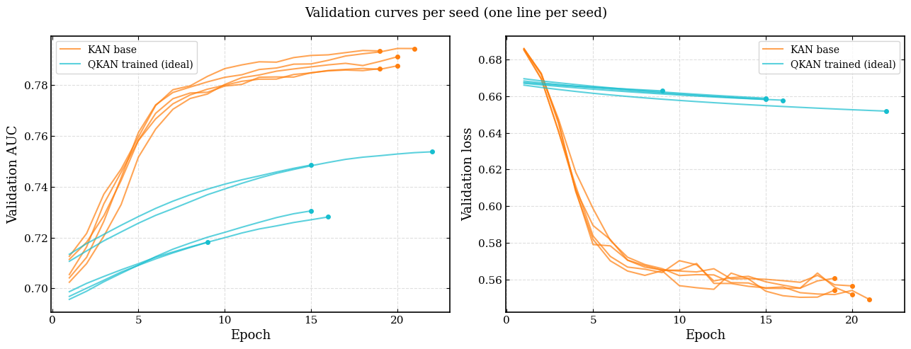
The per-seed validation curves show why the effect of fine-tuning is still modest. The base classical KAN converges in about 20 epochs, and its validation AUC levels off before early stopping. The QKAN behaves differently: its validation AUC grows almost linearly, about 0.003 per epoch, and is still rising when training stops, between epochs 9 and 22 out of a maximum of 50. Each epoch uses 1,000 samples with a batch size of 1,024, that is, a single optimization step, and the stopping criterion requires an improvement larger than $5\times10^{-3}$, more than one step gains. The QKAN is therefore undertrained, and its metrics should be read as a lower bound on what the circuit can reach. The validation loss barely moves (around 0.66, close to $\ln 2 \approx 0.693$) while AUC grows: with the logit bounded to $[-1, 1]$, even a perfect classifier could not push the cross-entropy below $\ln(1+e^{-1}) \approx 0.31$, so the loss is a weak signal of progress, while the ranking of events does improve.

The comparison across warm-start bases confirms the order Chebyshev > Sine > Random, both in AUC and in background rejection. The next figure shows the full background rejection ($1/\varepsilon_B$) versus signal efficiency curve for the same seven models. The order Chebyshev > Sine > Random holds along the entire curve, and the trained QKAN sits above its Chebyshev warm start and below the classical KANs.

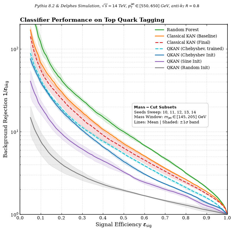
On these curves, initializing the circuit with the Chebyshev basis, with no further training, rejects roughly 2.4 times more background than random initialization at the 50% signal-efficiency working point ($\varepsilon_S=0.5$) (4.37 versus 1.81), with the sine basis at an intermediate point (3.26), consistent with its weaker edge fit. The gap grows at the more demanding working point, $\varepsilon_S=0.3$, where Chebyshev rejects about 3.6 times more background than the random control (10.4 versus 2.9). At $\varepsilon_S=0.9$ the gap closes (1.4 versus 1.1): this is the maximum signal-efficiency regime, where any classifier, including the random one, lets almost all background through.

To verify that these differences exceed the statistical noise of only five seeds, paired $t$-tests ($\alpha=0.05$) were run, with the null hypothesis that random initialization and each warm start give the same accuracy and AUC:

Comparison	Accuracy	AUC
Random vs Chebyshev	$t=-4.86$, $p=0.0082$	$t=-20.17$, $p=3.6\times10^{-5}$
Random vs Sine	$t=-5.00$, $p=0.0075$	$t=-17.95$, $p=5.7\times10^{-5}$

Both null hypotheses are clearly rejected, although the result should be read with caution since it rests on only five seeds.

Averaged over the five seeds, the quantum circuit’s accuracy hovers around 0.56-0.57, versus ~0.70 for the classical KAN, with recall ~0.97 and precision ~0.54 (0.98 and 0.53 in the reference run). The ranking signal, as measured by AUC, is preserved, but the fixed threshold of 0.5 is poorly calibrated for the circuit’s output.

The next figure shows the confusion matrices normalized by true class (each row sums to 1), with the mean and standard deviation over the five seeds. Each seed has the same number of signal and background jets in its test set (4,733 per class), so the rates of the different seeds are directly comparable.

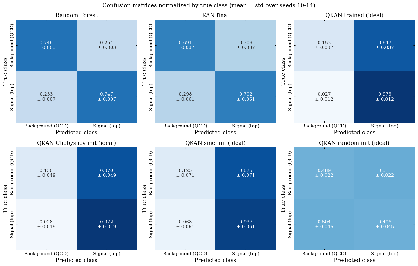
The Random Forest and the final KAN have nearly symmetric matrices (~0.75 on the diagonal for the Random Forest and ~0.69-0.70 for the final KAN), so their errors are spread across both classes and their accuracy agrees with their AUC. The QKAN, both with the Chebyshev and sine initializations and after training, correctly classifies more than 97% of top jets, but only between 13% and 15% of QCD jets. Since the output $\langle Z \rangle \in [-1,1]$ is used as a logit, the probabilities stay in practice within ~[0.48, 0.72], and almost every event falls above the 0.5 threshold. Training barely improves the true negative rate (from 0.130 to 0.153): it reorders the events, which raises the AUC, without moving them across the threshold. The random initialization sits near 0.5 in all four cells, the behavior of a chance-level classifier. For this reason AUC is reported as the main metric instead of accuracy.

9. Comparison with the literature

The reference paper for this benchmark, Kasieczka et al. (2019), and the most-cited comparison notebook that reproduces and extends its figures, SebastianMacaluso/TopTagComparison, gather 12 classical and deep-learning taggers (ParticleNet, TreeNiN, ResNeXt, PFN, CNN, NSub, LBN, P-CNN, LoLa, EFN, EFP, TopoDNN) plus the GoaT meta-tagger, evaluated on the full dataset of 2 million jets with no mass restriction. In the original table (“single model”), AUC ranges from 0.955 (LDA, the weakest tagger, explicitly excluded from the meta-tagger for contributing no signal) to 0.985 (ParticleNet); excluding LDA, the range is 0.972 (TopoDNN) to 0.985 (ParticleNet). Background rejection at $\varepsilon_S=0.3$ ranges, in the same table, from 295 ± 14 (LDA) to 1412 ± 46 (ParticleNet).

This comparison requires an explicit caveat: those numbers use the full dataset, with no cuts, while all of this project’s results correspond to the aggressive mass-cut regime (145-205 GeV), designed to remove the easiest cue and force models to rely on substructure. The figures are therefore not comparable point by point: the Random Forest’s AUC of 0.823 and the trained QKAN’s 0.736 are obtained on a deliberately harder problem than the one in the reference table. A direct comparison requires evaluating the same pipeline without the mass cut and with replicas, which remains as future work.

Beyond the mass cut, two factors widen this gap. The first is variable compression: pruning reduces 22 variables to just 2, while architectures such as ParticleNet or IAFormer consume the full constituent cloud with graphs or sparse attention designed for that high dimensionality. The second, identified when revisiting the preprocessing after obtaining the main results, is that each jet carries up to 200 constituents and the pipeline only uses the 10 most energetic. This deliberate simplification keeps the circuit simulable, but it leaves out almost all low-energy substructure, precisely where architectures such as IAFormer (Esmail et al., 2026) or the Lorentz-equivariant L-GATr (Brehmer et al., 2025) report gains. Together with the mass cut and the compression to two variables, it is a third reason for the gap with the state of the art.

10. Related work: other quantum-KAN approaches

Other efforts combine KANs with quantum computing. This section situates the project against three of them, each of which addresses the same bottleneck (how to quantize a learnable univariate function) with a different strategy.

QKAN (Ivashkov et al., 2024) is the theoretical proposal that motivated, from the outset, the search for an alternative that could run on noisy hardware. It implements a KAN’s univariate functions through block encoding and the Quantum Singular Value Transformation (QSVT). This gives it strong expressivity guarantees, but ties it to fault-tolerant primitives that no current NISQ device can run natively. It represents the theoretical ceiling against which any QKAN designed for current hardware is measured: it offers stronger guarantees, but it cannot be executed today.

Ria Khatoniar’s QKAN project (Khatoniar, 2025a, 2025b; GSoC 2025, also at ML4SCI) is the closest precedent in time and the one that directly inspired the choice of the sine basis in this work. Her first report describes a hybrid QKAN combining QSVT encoding, a quantum linear combination of unitaries (LCU), and a Hadamard test for summation, with a classical KAN/SineKAN-style readout; it explicitly reports that the architecture could not scale beyond a certain point on the quark-gluon dataset, due to simulator memory failures (kernel crashes). Her second report presents a fully quantum KAN based on a Quantum Circuit Born Machine (QCBM), with label and position qubits, an entangling layer (LabelMixer), and Pauli-Z/X readout; there she states that extending the approach to quark-gluon tagging or jet-mass prediction “could not yet be achieved, mainly because the current architecture is computationally slow”, limiting it to simulators. Both reports conclude by signaling an intent to continue in the future. This project picks up that direction in choosing the sinusoidal basis for the warm start, using the SineKANLayer code from her repository as a direct reference.

QuKAN (Werner et al., 2025) explores an approach different from that of Ivashkov et al. despite the similar name: instead of encoding each univariate function through QSVT, it directly uses a Quantum Circuit Born Machine as a generative mechanism to represent them, quantum from the start and without distilling an already-trained classical KAN.

Taken together, the four projects (Ivashkov et al., Khatoniar, Werner et al., and this work) show a clear pattern: scaling a quantum KAN beyond a handful of variables is, in 2025-2026, a shared open problem. The causes are the reliance on fault-tolerant primitives (Ivashkov et al.), simulation memory (Khatoniar), the cost of a generative quantum mechanism (Werner et al.), or, in this case, the need to prune aggressively before the circuit can be simulated. None of the four has yet demonstrated a QKAN running without compromises on a full-scale HEP dataset.

11. Conclusions

Five conclusions summarize the project.

1. Classical pruning works as a qubit filter. The KAN reduces 22 inputs to two variables (mass and multiplicity) and 10 or 11 qubits depending on the seed, and the circuit still reaches an AUC of ~0.73 with the mass cut.
2. The warm start carries real information. The order Chebyshev > Sine > Random is consistent across seeds and statistically significant over five replicas. Random initialization performs at chance level (AUC ~0.49), showing that topology alone is not enough. The Chebyshev basis is superior because its per-edge fit is much closer to the real classical response (mean $R^2$ of 0.998, versus ~0.56 for the sine basis).
3. Simulated noise has a small effect. The gap between the ideal and noisy backends is at most ~0.006 AUC. The result is encouraging, but it comes from a simulated noise model and still needs to be validated on real hardware. In addition, simulating it is costly: evaluating the noisy backend takes on average ~18 times longer than ideal.
4. The mass cut defines a deliberately hard problem. Removing the easy mass cue forces the models to rely on substructure, which the two surviving variables capture only partially. For this reason the project’s figures are not comparable point by point with those in the literature, which are obtained without the cut.
5. The classical ceiling is set by the Random Forest. It has access to all 22 variables and leads on every metric; the quantum model does not surpass it. The value of the hybrid approach lies in producing a compact, interpretable circuit that preserves a considerable fraction of that performance.

12. Contributions

• A reproducible, regime-aware pipeline: the different regimes are encoded in the directory structure, replica subsets are class-balanced, each stage is idempotent via checkpoints, and results across several seeds are collected into a single Parquet table.
• HEPKAN, a subclass of pykan that fixes a serialization bug in input pruning and reduces plotting and logging overhead.
• A pruning rule designed specifically for quantum limits, combining attribution thresholds with a hard fan-in cap.
• A classical-to-quantum bridge: the extractor converts a pruned KAN into a sum/multiplication graph, and the QKAN builder converts that graph into a PennyLane circuit.
• Two interchangeable bases plus a control, allowing the value of the warm start to be measured across three simulation backends, evaluated before and after training.
• A diagnosed and fixed bug: the adaptive Chebyshev degree search was silently collapsing the reference AUC on smaller datasets; the cause was identified and replaced with a fixed degree.
• A classical benchmark, the Random Forest, evaluated with the same metrics and the same data split.
• An exploratory analysis documenting the dataset layout, the $\Delta R$ artifact, and the choice of 10 constituents and 22 inputs.

13. Limitations and future work

• Few replicas: the statistical tests use five seeds, and each seed uses its own subset, so the effect of the seed and that of the subset cannot be separated.
• Mass-cut regime only: the pipeline still needs to be evaluated without the mass cut and with replicas, which would allow a direct comparison with the literature.
• Extreme compression: pruning leaves ~2 input variables; relaxing it pushes the qubit count beyond what is simulable in reasonable time.
• Only the 10 most energetic constituents out of up to 200 per jet: an additional restriction that likely discards relevant low-energy substructure.
• Undertraining: each QKAN epoch is a single optimization step and the early-stopping threshold is coarse, so training stops while validation AUC is still improving.
• Calibration: quantum accuracy and precision are weak even where AUC is good; a tuned decision threshold remains to be studied.
• Sine basis: adding a constant term to the least-squares fit raises its $R^2$ above that of Chebyshev, confirming that the lack of this term was the cause of the original poor $R^2$. However, this verification was limited to the edge-level fit: the full circuit with the extended basis still needs to be run to determine whether this better fit actually translates into a higher warm start AUC than Chebyshev, or if something is lost in the rotation angle encoding.
• Simulated and partial noise only: FakeManilaV2 approximates a real device, but it is not one; and since that device has 5 qubits compared to the 11 in the circuit, the calibrated noise only covers the first 5, the rest of the circuit runs ideally even on the noisy backend. Extending the noise model to all 11 qubits, or repeating the experiment with a reference device of comparable size, is an obvious step before drawing firm conclusions about noise tolerance, considering the significant increase in time that this fully noisy and simulated approach would entail, which remains pending.
• Depth-2 networks only: deeper KANs would require intermediate measurement and re-encoding. Stacking more re-uploading layers without that redesign is technically difficult and increases the barren plateau risk, so this direction depends on first solving intermediate measurement.
• Other datasets: a preprocessing pipeline exists for quark-gluon tagging.

In sum, the project shows that a classical KAN can decide the shape of a quantum circuit, that knowledge transferred through a good basis has a measurable effect, and that the resulting compact model preserves a useful part of the classification signal. The model does not yet match the best classical baseline, and that limit is reported alongside the results.

Acknowledgements

I want to thank my friend Eduardo Villamil for providing computational resources for this project, ML4SCI for the opportunity to take part in Google Summer of Code 2026, and all the admins, mentors, and members of the program for their useful feedback throughout the project.

---

References

1. Arias Alamo, D., Hernández López, S., & Lázaro González, J. (2025). Is data-reuploading really a cheat code? An experimental analysis. In Proceedings of the 1st International Conference on Quantum Software (IQSOFT 2025). https://doi.org/10.5220/0013555000004525
2. Brehmer, J., Bresó, V., de Haan, P., Plehn, T., Qu, H., Spinner, J., & Thaler, J. (2025). A Lorentz-equivariant transformer for all of the LHC. SciPost Physics. https://arxiv.org/abs/2411.00446
3. Esmail, W., Hammad, A., & Nojiri, M. (2026). IAFormer: Interaction-aware transformer network for collider data analysis. SciPost Physics, 20, Article 108. https://arxiv.org/abs/2505.03258
4. Gleyzer, S., Nguyen, H., Ramakrishnan, D. P., & Reinhardt, E. A. F. (2025). Sinusoidal approximation theorem for Kolmogorov–Arnold networks. Mathematics, 13(19), Article 3157. https://doi.org/10.3390/math13193157
5. Ivashkov, P., Huang, P.-W., Koor, K., Pira, L., & Rebentrost, P. (2024). QKAN: Quantum Kolmogorov-Arnold networks with applications in machine learning and multivariate state preparation. arXiv. https://arxiv.org/abs/2410.04435. Published in 2026 in npj Quantum Information. https://doi.org/10.1038/s41534-026-01202-5
6. Kasieczka, G., Plehn, T., Thompson, J., & Russell, M. (2019). Top quark tagging reference dataset (Version v0) [Data set]. Zenodo. https://doi.org/10.5281/zenodo.2603256. See also the associated paper: Kasieczka, G., et al. (2019). The Machine Learning landscape of top taggers. SciPost Physics, 7, 014. https://arxiv.org/abs/1902.09914
7. Khatoniar, R. (2025a). GSoC 2025 | Quantum Kolmogorov-Arnold networks for high energy physics analysis at the LHC (Part I) [Blog post]. Medium. https://medium.com/@riakhatoniar1234/gsoc-2025-quantum-kolmogorov-arnold-networks-for-high-energy-physics-analysis-at-the-lhc-a98207bf6d4c
8. Khatoniar, R. (2025b). GSoC 2025 | Quantum Kolmogorov-Arnold networks for high energy physics analysis at the LHC (Part II) [Blog post]. Medium. https://medium.com/@riakhatoniar1234/gsoc-2025-quantum-kolmogorov-arnold-networks-for-high-energy-physics-analysis-at-the-lhc-part-8b44f5616e6f
9. Liu, Z., Wang, Y., Vaidya, S., Ruehle, F., Halverson, J., Soljačić, M., Hou, T. Y., & Tegmark, M. (2024). KAN: Kolmogorov-Arnold networks. arXiv. https://arxiv.org/abs/2404.19756
10. Liu, Z., Ma, P., Wang, Y., Matusik, W., & Tegmark, M. (2024). KAN 2.0: Kolmogorov-Arnold networks meet science. arXiv. https://arxiv.org/abs/2408.10205
11. Macaluso, S. (n.d.). TopTagComparison [Code repository]. GitHub. Retrieved September 21, 2026, from https://github.com/SebastianMacaluso/TopTagComparison
12. Reinhardt E, Ramakrishnan D and Gleyzer S (2025) SineKAN: Kolmogorov-Arnold Networks using sinusoidal activation functions. Front. Artif. Intell. 7:1462952. doi: 10.3389/frai.2024.1462952
13. Sidharth, S. S., Gokul, R., Anas, K. P., & Keerthana, A. R. (2024). Chebyshev polynomial-based Kolmogorov-Arnold networks: An efficient architecture for nonlinear function approximation. arXiv. https://arxiv.org/abs/2405.07200
14. Werner, Y., Malemath, A., Liu, M., Fortes Rey, V., Palaiodimopoulos, N., Lukowicz, P., & Kiefer-Emmanouilidis, M. (2025). QuKAN: A quantum circuit Born machine approach to quantum Kolmogorov Arnold networks. Scientific Reports, 15. https://doi.org/10.1038/s41598-025-22705-9

Dataset: Zenodo record 2603256 (top tagging, Pythia8 + Delphes ATLAS). This project builds on the original proposal submitted to GSoC 2026 / ML4SCI, “Quantum Sine-Kolmogorov-Arnold Networks for High Energy Physics Analysis” (Toral, J., 2026).